John L. Godlee

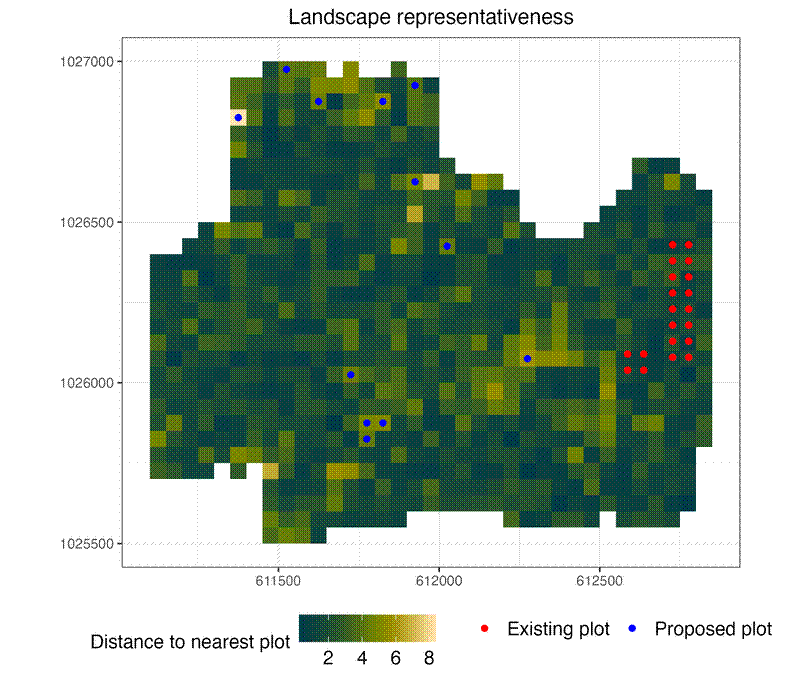
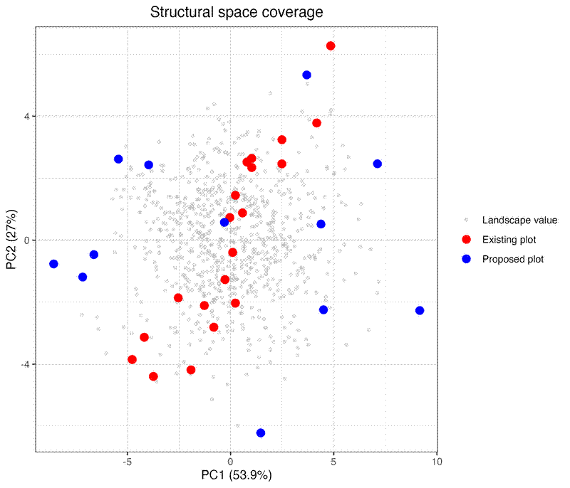
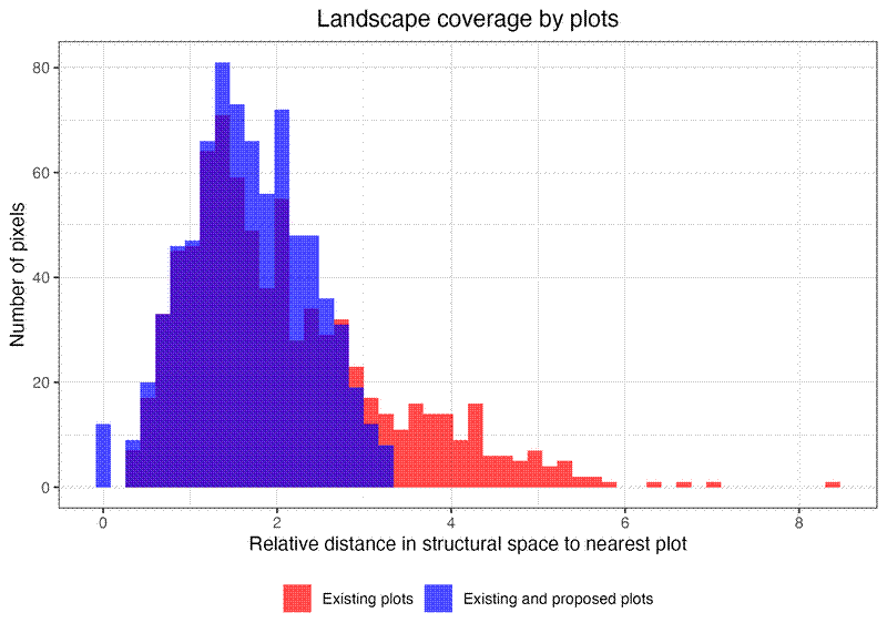
In the GEO-TREES project we are developing sites across tropical forests to calibrate and validate biomass maps, using a combination of airborne LiDAR (ALS), terrestrial LiDAR (TLS), and tree inventory data from permanent sample plots. We use the airborne LiDAR to scale up biomass estimates from the permanent plots across the landscape, by fitting a site-specific model which predicts biomass from forest structure (canopy height, canopy density, etc). To fit a model with good predictive power we need to have plots which cover the diversity of forest structural types found across the site. Most of the GEO-TREES sites already have some plots, but it’s important to assess whether those plots are representative of the structural diversity found across the plots.

I’ve written some code which (1) does an assessment of the structural diversity of the site from ALS data, (2) determines the extent to which existing plots within the site represent the structural diversity of the site, and (3) recommends locations for new plots which fill gaps in the coverage of the structural diversity of the site.

First, load packages:

# How representative of forest structure are plots in a site?
# John L. Godlee (johngodlee@gmail.com)
# Last updated: 2025-09-04

# Purpose:
# To what extent are existing plots representative of the broader landscape forest structure? 
# Identify optimal locations for new plots to fill gaps in multidimensional forest structure space.

# Load required libraries
library(dplyr)
library(tidyr)
library(ggplot2)
library(patchwork)
library(terra)
library(sf)
library(plotly)  # Interactive 3D plots
library(FNN)  # Nearest neighbor analysis
library(scico)  # Color palettes
library(lhs)  # Latin-hypercube sampling

Then I define extract_plot_metrics() to extract structural metrics from the ALS for each of the existing plots:

# Extract values from raster across polygons
#
# @param r raster
# @param p_sf sf object containing plot polygons 
# @param plot_id column name of plot IDs in `p_sf` 
#
# @return dataframe containing extracted metrics for each polygon
# 
extract_plot_metrics <- function(r, p_sf, plot_id = "plot_id", fun = mean, ...) {

  # Extract metrics for each plot polygon
  out <- terra::extract(r, vect(p_sf), fun = fun, 
    na.rm = TRUE, ID = FALSE, ...)
  
  # Add plot IDs
  out <- cbind(p_sf[[plot_id]], out)
  names(out)[1] <- plot_id

  # Add XY coordinates of centroids
  coords <- as.data.frame(st_coordinates(st_centroid(p_sf)))
  names(coords) <- c("x", "y")
  out <- cbind(out, coords)

  # Return
  return(out)
}

Then I define analyse_repres() which runs a principal component analysis of the structural metrics across the site and places the existing plots in PCA-space.

# Run a PCA on the landscape structural metrics, and place plots in that space
# Get nearest neighbour distance from each landscape pixel to plots
# Return dataframe with metrics of plot coverage
# 
# @param r raster 
# @param p dataframe containing structural metrics for each plot, as returned
#     by `extract_plot_metrics()`
# @param n_pca number of PCA axes used in analysis
#
# @return list containing: `r_df`: pixel values, `p_df`: plot values, `r_pca`:
#     PCA object from pixel values, `p_pca` plot values in PCA space,
#     `nn_dist_mean`, `nn_dist_max`, `nn_dist_q95`: mean, max and 95th
#     percentile structural distance of pixels to nearest plot across the
#     landscape, `coverage_score`: `1 - (mean(nn) / max(nn)`
# 
analyse_repres <- function(r, p, n_pca = 3) {
  # Convert raster to data frame for landscape
  r_df <- as.data.frame(r, xy = TRUE, na.rm = TRUE)
  
  # Select only metric columns 
  metric_cols <- names(r_df)[!names(r_df) %in% c("x", "y")]
  
  # Standardize metrics
  r_sc <- scale(r_df[,metric_cols])
  p_sc <- scale(p[,metric_cols])
  
  # PCA to reduce dimensionality
  r_pca <- prcomp(r_sc, scale = FALSE)
  
  # Project plots into PCA space
  p_pca <- predict(r_pca, p_sc)
  
  # Calculate nearest neighbor distances
  # For each landscape pixel, find distance to nearest plot
  nn <- get.knnx(p_pca[, 1:n_pca], r_pca$x[, 1:n_pca], k = 1)$nn.dist[,1]
  
  # Add distances back to landscape dataframe
  r_df$nn_dist <- nn
  r_df <- cbind(r_df, r_pca$x[,1:n_pca])

  # Add PCA values 
  p_df <- p
  p_df <- cbind(p_df, p_pca[,1:n_pca])
  
  # Create representativeness metrics
  out <- list(
    r_df = r_df,
    p_df = p_df,
    r_pca = r_pca,
    p_pca = p_pca,
    nn_dist_mean = mean(nn),
    nn_dist_max = max(nn),
    nn_dist_q95 = quantile(nn, 0.95),
    coverage_score = 1 - (mean(nn) / max(nn))
  )
  
  # Return
  return(out)
}

Then I define identify_optimal_plots() to identify potential locations for new plots which most optimally fill gaps in PCA-space. This function allows different gap-filling algorithms:

maximin_select() - iteratively proposes new plots in pixels with structural attributes furthest away from the existing (and previously proposed) plots.
minimax_select() - minimizes the maximum distance of any pixel to its nearest plot in PCA space.
lhs_select() - latin-hypercube sampling. Optimises for uniform coverage across PCA space.

# Define function for latin-hypercube sampling 
lhs_select <- function(r_df, n_plots, n_pca, min_dist) {
  # Scale PCs to [0,1] for uniform LHS sampling
  pcs <- r_df[, paste0("PC", 1:n_pca)]
  pcs_scaled <- scale(pcs,
    center = apply(pcs, 2, min),
    scale  = apply(pcs, 2, max) - apply(pcs, 2, min))
  
  # Generate LHS design
  lhs_design <- randomLHS(n_plots, n_pca)
  
  # Prepare candidates
  cand <- r_df
  cand$id <- seq_len(nrow(cand))
  plots_sel <- data.frame()
  
  for (i in seq_len(n_plots)) {
    # LHS target point
    target <- lhs_design[i, ]
    
    # Compute distance from all candidates to LHS target
    dists <- rowSums((pcs_scaled - matrix(target, nrow(cand), 
      n_pca, byrow=TRUE))^2)
    
    # Filter by spatial distance to already-selected plots
    if (nrow(plots_sel) > 0) {
      dists_spat <- get.knnx(
        plots_sel[, c("x","y")],
        cand[, c("x","y")],
        k = 1
      )$nn.dist[,1]
      valid_cand <- which(dists_spat > min_dist)
    } else {
      valid_cand <- seq_len(nrow(cand))
    }
    
    if (length(valid_cand) > 0) {
      # Select candidate closest to the LHS target
      best_idx <- valid_cand[which.min(dists[valid_cand])]
      new_plot <- cand[best_idx, ]
    } else {
      warning(paste("Could not find valid location for plot", i))
      next
    }
    
    # Append proposed plot
    plots_sel <- rbind(plots_sel, new_plot)
    
    # Remove selected location from candidates
    cand <- cand[cand$id != new_plot$id, ]
    pcs_scaled <- pcs_scaled[-new_plot$id, , drop = FALSE]
  }
  
  # Return
  return(plots_sel)
}

# Define function for maximin sampling 
maximin_select <- function(r_df, n_plots, n_pca, min_dist) {
  # Maximin: maximize the minimum distance to existing plots
  cand <- r_df[order(r_df$nn_dist, decreasing = TRUE),]
  cand$id <- seq_len(nrow(cand))
  
  # Iteratively add plots 
  plots_sel <- data.frame()
  for (i in seq_len(n_plots)) {
    if (nrow(plots_sel) == 0) {
      # First plot: choose furthest from existing plots
      new_plot <- cand[1,]
    } else {
      # Re-calculate minimum distance between new plots and pixels 
      dist_sel <- get.knnx(
        plots_sel[,paste0("PC", 1:n_pca)], 
        cand[,paste0("PC", 1:n_pca)], 
        k = 1)$nn.dist[,1]
      
      # Combine with distance to existing plots
      comb_score <- pmin(cand$nn_dist, dist_sel)
      
      # Calculate minimum spatial distance between new plots and pixels 
      dists_spat <- get.knnx(
        plots_sel[, c("x", "y")],
        cand[, c("x", "y")],
        k = 1)$nn.dist[,1]
      
      # Filter to plots a minimum spatial distance away from other proposed plots
      valid_cand <- which(dists_spat > min_dist)
      
      # Select candidate with maximum combined score
      if (length(valid_cand) > 0) {
        best_idx <- valid_cand[which.max(comb_score[valid_cand])]
        new_plot <- cand[best_idx, ]
      } else {
        warning(paste("Could not find valid location for plot", i))
        next
      }
    }
    
    # Append proposed plot
    plots_sel <- rbind(plots_sel, new_plot)

    # Remove selected location from cand
    cand <- cand[cand$id != new_plot$id,]
  }

  # Return
  return(plots_sel)
}

# Define function for minimax sampling 
minimax_select <- function(r_df, n_plots, n_pca, min_dist) {
  # Minimax: minimize the maximum distance from any pixel to the nearest plot
  cand <- r_df[order(r_df$nn_dist, decreasing = TRUE),]
  cand$id <- seq_len(nrow(cand))
  
  # Iteratively add plots
  plots_sel <- data.frame()
  for (i in seq_len(n_plots)) {
    if (nrow(plots_sel) == 0) {
      # First plot: choose furthest from existing plots
      new_plot <- cand[1, ]
    } else {
      # Re-calculate minimum distance between new plots and pixels 
      dist_sel <- get.knnx(
        plots_sel[, paste0("PC", 1:n_pca)], 
        cand[, paste0("PC", 1:n_pca)], 
        k = 1)$nn.dist[, 1]
      
      # Effective nearest distance for each candidate
      comb_score <- pmin(cand$nn_dist, dist_sel)
      
      # Calculate max distance if each candidate were added
      # Lower is better (minimax criterion)
      max_dists <- sapply(seq_len(nrow(cand)), function(j) {
        test_sel <- rbind(plots_sel, cand[j,])
        test_dists <- get.knnx(
          test_sel[, paste0("PC", 1:n_pca)],
          cand[, paste0("PC", 1:n_pca)],
          k = 1)$nn.dist[,1]
        max(test_dists)
      })
      
      # Enforce spatial separation
      dists_spat <- get.knnx(
        plots_sel[,c("x", "y")],
        cand[, c("x", "y")],
        k = 1)$nn.dist[, 1]
      valid_cand <- which(dists_spat > min_dist)
      
      # Select candidate that minimizes the maximum distance
      if (length(valid_cand) > 0) {
        best_idx <- valid_cand[which.min(max_dists[valid_cand])]
        new_plot <- cand[best_idx, ]
      } else {
        warning(paste("Could not find valid location for plot", i))
        next
      }
    }
    
    # Append proposed plot
    plots_sel <- rbind(plots_sel, new_plot)
    
    # Remove selected location from cand
    cand <- cand[cand$id != new_plot$id,]
  }
  
  # Return
  return(plots_sel)
}

# Iteratively add locations which most efficiently fill the structural space
#
# @param repr object returned by `analyse_repres()`
# @param n_plots maximum number of new plots to add
# @param n_pca number of PCA axes used in analysis
# @param min_dist minimum spatial distance between new plots
# @param method either "maximin", "minimax" or "lhs" to choose a gap-filling
#     algorithm
# @param elbow logical, if TRUE then plots are iteratively added up to
#     `n_plots` to determine the reduction in mean structural distance across
#     the landscape
#
# @details
# `method`: "maximin" iteratively proposes new plots in pixels with structural
#     attributes furthest away from the existing (and previously proposed)
#     plots. "minimax" aims to minimize the maximum distance of any pixel to
#     its nearest plot in PCA space. "lhs" (latin-hypercube sampling) doesn’t
#     focus on distances between points directly, instead it optimises for
#     uniform coverage across PCA space.
#
# @return dataframe containing locations and structural metrics for proposed
#     new plots, ordered by largest reduction in mean structural distance of
#     pixels to nearest plots
# 
identify_optimal_plots <- function(repr, n_plots = 10, n_pca = 3, min_dist = 0, method = "maximin", elbow = FALSE) {
  
  # Extract dataframes
  r_df <- repr$r_df
  p_df <- repr$p_df
  

  if (method == "maximin") {
    plots_sel <- maximin_select(r_df, n_plots, n_pca, min_dist)
  } else if (method == "minimax") { 
    plots_sel <- minimax_select(r_df, n_plots, n_pca, min_dist)
  } else if (method == "lhs") { 
    plots_sel <- lhs_select(r_df, n_plots, n_pca, min_dist)
  } else {
    stop("'method' must be one of 'maximin', 'minimax' or 'lhs'")
  }

  # Remove ID value
  plots_sel <- plots_sel[,!names(plots_sel) == "id"]

  # Optionally create elbow plot to find optimal number of new plots
  if (elbow) {
    elbow_dist <- c()
    # Iteratively add new plots to plot data
    for (i in 0:n_plots) {
      pca_comb <- rbind(
        p_df[,paste0("PC", 1:n_pca)], 
        plots_sel[1:i,paste0("PC", 1:n_pca)])

      # Calculate mean distance between pixels and plots (old and new) 
      nn <- get.knnx(pca_comb, r_df[,paste0("PC", 1:n_pca)], k = 1)$nn.dist[,1]
      elbow_dist[i+1] <- mean(nn) 
    }

    # Create pretty dataframe
    elbow_df <- data.frame(
      new_plots = 0:n_plots,
      nn_dist_mean = elbow_dist)

    # Create bar plot
    p <- ggplot(data = elbow_df, aes(x = new_plots, y = nn_dist_mean)) + 
      geom_col() + 
      theme_bw() + 
      scale_x_continuous(breaks = seq(0, n_plots)) + 
      labs(
        x = "Number of additional plots",
        y = "Mean relative distance in structural space to nearest plot") + 
      coord_cartesian(ylim = c(
        min(elbow_df$nn_dist_mean), 
        max(elbow_df$nn_dist_mean)))

    return(list(p, elbow_df))
  }

  # Return
  return(plots_sel)
}

And finally I define plot_repres() to visualise the results of the analysis:

# Visualise outputs of representivity analysis
#
# @param repr object returned by `analyse_repres()`
# @param plots_sel optional, object returned by `identify_optimal_plots()`
#
# @return plots to visualise plots in structural space. `map` shows the
#     location of plots and the structural distance of each pixel in the
#     landscape to its nearest plot, if `plots_sel` is provided this includes
#     the proposed new plots. `pca2d` scatter plot of the first two PCA axes
#     of structural metrics. `pca3d` an interactive (plotly) 3D scatter plot of
#     the first three PCA axes of structural metrics. `hist` (only returned if
#     `plots_sel` is provided) histograms showing the distance in structural
#     PCA space from each pixel to its nearest plot, comparing the distribution
#     when using only existing plots to the distribution when including the
#     proposed new plots.
# 
plot_repres <- function(repr, plots_sel = NULL) {

  # Extract dataframes
  r_df <- repr$r_df
  p_df <- repr$p_df
  
  # Map of representativeness (multi-dimensional distance to nearest plot)
  p_old <- p_df[,c("x", "y")] 
  p_old$type <- "Existing plot"
  if (!is.null(plots_sel)) { 
    p_new <- plots_sel[,c("x", "y")] 
    p_new$type <- "Proposed plot"
    p_all <- rbind(p_old, p_new)
  } else {
    p_all <- p_old
  }

  # Define legend items 
  size_map <- c("Existing plot" = 3, "Proposed plot" = 3, "Landscape value" = 1)
  opacity_map <- c("Existing plot" = 1, "Proposed plot" = 1, "Landscape value" = 0.4)
  colour_map <- c("Existing plot" = "red", "Proposed plot" = "blue", "Landscape value" = "grey")
  shape_map <- c("Existing plot" = "circle", "Proposed plot" = "circle", "Landscape value" = "circle")

  p1 <- ggplot() +
    geom_raster(data = r_df, aes(x = x, y = y, fill = nn_dist)) +
    scale_fill_scico(name = "Distance to nearest plot", palette = "bamako") +
    geom_point(data = p_all, 
      aes(x = x, y = y, shape = type, colour = type)) + 
    scale_colour_manual(name = NULL, 
      values = colour_map) + 
    scale_shape_manual(name = NULL, 
      values = shape_map) + 
    coord_equal() +
    theme_bw() +
    ggtitle("Landscape representativeness") +
    labs(
      x = NULL, 
      y = NULL) + 
    theme(
      plot.title = element_text(hjust = 0.5),
      legend.position = "bottom",
      legend.title = element_text(size = 12),
      legend.text = element_text(size = 12))
  
  # Extract variance explained by each PCA axis
  pca_var <- summary(repr$r_pca)$importance[2, 1:3] * 100

  pca_pt_r <- as.data.frame(repr$r_pca$x[,1:3])
  pca_pt_r$type <- "Landscape value" 
  pca_pt_p <- as.data.frame(repr$p_pca[,1:3])
  pca_pt_p$type <- "Existing plot" 
  if (!is.null(plots_sel)) {
    pca_pt_n <- plots_sel[,paste0("PC", 1:3)]
    pca_pt_n$type <- "Proposed plot" 
    pca_pt_all <- rbind(pca_pt_r, pca_pt_p, pca_pt_n)
  } else {
    pca_pt_all <- rbind(pca_pt_r, pca_pt_p) 
  }
  pca_pt_all$type <- factor(pca_pt_all$type, 
    levels = c("Landscape value", "Existing plot", "Proposed plot"))
  
  p2 <- ggplot() +
    geom_point(data = pca_pt_all, 
      aes(x = PC1, y = PC2, 
        size = type, shape = type, colour = type, alpha = type)) + 
    scale_size_manual(name = NULL, values = size_map) + 
    scale_colour_manual(name = NULL, values = colour_map) + 
    scale_shape_manual(name = NULL, values = shape_map) + 
    scale_alpha_manual(name = NULL, values = opacity_map) + 
    xlab(paste0("PC1 (", round(pca_var[1], 1), "%)")) +
    ylab(paste0("PC2 (", round(pca_var[2], 1), "%)")) +
    theme_bw() +
    ggtitle("Structural space coverage") +
    theme(plot.title = element_text(hjust = 0.5))
  
  # 3D PCA plot
  p3 <- plot_ly(type = "scatter3d", mode = "markers") %>% 
    layout(
      title = "Structural space coverage",
      scene = list(
        xaxis = list(title = paste0("PC1 (", round(pca_var[1], 1), "%)")),
        yaxis = list(title = paste0("PC2 (", round(pca_var[2], 1), "%)")),
        zaxis = list(title = paste0("PC3 (", round(pca_var[3], 1), "%)"))
      )
    )

  for (t in unique(pca_pt_all$type)) {
    subset_pca_pt_all <- pca_pt_all[pca_pt_all$type == t,]
  
    p3 <- add_trace(
      p3,
      data = subset_pca_pt_all,
      x = ~PC1, y = ~PC2, z = ~PC3,
      name = t,
      marker = list(
        size = size_map[t],
        opacity = opacity_map[t],
        color = colour_map[t],
        symbol = shape_map[t],
        line = list(width = 1, color = "black")
      )
    )
  }
  
  # Coverage improvement analysis
  if (!is.null(plots_sel)) {
    # Recalculate distances with new plots
    all_plots_pca <- rbind(
      repr$p_pca[,paste0("PC", 1:3)],
      as.matrix(plots_sel[,paste0("PC", 1:3)])
    )
    
    nn_new <- get.knnx(all_plots_pca, repr$r_pca$x[,paste0("PC", 1:3)], k = 1)
    
    # Create dataframe
    improvement_df <- data.frame(
        orig = repr$r_df$nn_dist,
        with_new = nn_new$nn.dist[, 1]) %>%
      pivot_longer(
        everything(), 
        names_to = "scenario", 
        values_to = "distance") %>% 
      mutate(scenario = factor(scenario, 
        levels = c("orig", "with_new"),
        labels = c("Existing plots", "Existing and proposed plots")))
    
    p4 <- ggplot(improvement_df, aes(x = distance, fill = scenario)) +
      geom_histogram(alpha = 0.7, position = "identity", bins = 50) +
      scale_fill_manual(name = NULL, 
        values = c("Existing plots" = "red", "Existing and proposed plots" = "blue")) +
      theme_bw() +
      ggtitle("Landscape coverage by plots") +
      labs(
        x = "Relative distance in structural space to nearest plot",
        y = "Number of pixels") + 
      theme(
        plot.title = element_text(hjust = 0.5),
        legend.position = "bottom")

    return(list(map = p1, pca2d = p2, pca3d = p3, hist = p4))
  }
  
  return(list(map = p1, pca2d = p2, pca3d = p3))
}

Here is a worked example with the latin-hypercube sampling:

# Import ALS metrics
als <- rast("./als.tiff")

# Import 50x50 m plot polygons
subplots <- st_read("./plots.gpkg")

# Filter subplots to ALS data
als_poly <- st_as_sf(as.polygons(als, na.rm = TRUE))
subplots_als <- st_join(subplots, als_poly, join = st_intersects) %>% 
  filter(!is.na(pulse_density)) 

# Only include bottomleft subplots
subplots_fil <- subplots_als %>% 
  filter(grepl("bottomleft", subplot_id))

# Select relevant metrics from ALS data
# names(als)
als_sel <- als[[c(
  "zmax.canopy.vox",
  "zmean.canopy.vox",
  "zcv.canopy.vox",
  "zskew.canopy.vox",
  "zkurt.canopy.vox",
  "zq10.canopy.vox",
  "zq30.canopy.vox",
  "zq50.canopy.vox",
  "zq70.canopy.vox",
  "zq90.canopy.vox",
  "lad_cv.aboveground.vox",
  "lad_sum.aboveground.vox")]]

# Extract metrics from raster
p_ext <- extract_plot_metrics(als_sel, subplots_fil, 
  plot_id = "subplot_id", fun = mean)

# Analyse representivity of plots
repr <- analyse_repres(als_sel, p_ext, n_pca = 3)

# Explore the optimal number of new plots
identify_optimal_plots(repr, n_plots = 50, method = "maximin", elbow = TRUE)

# Find optimal plots
optimal_plots_maximin <- identify_optimal_plots(repr, n_plots = 12, 
  method = "maximin")

# Visualize
plots_vis <- plot_repres(repr, optimal_plots_maximin)

plots_vis$map 

plots_vis$pca2d

plots_vis$hist

Map showing structural diversity of the site with existing and suggested new plots.

PCA plot with existing plots, suggested new plots, and pixels across the landscape.

Histograms showing the structural distance of pixels to their most similar plot, using only existing plots (red) and also including new suggested plots (blue)

Filling gaps in plot coverage across a landscape based on forest structure

2025-09-06