I have been reading field data collection protocols from various networks of permanent forest tree monitoring plots to come up with recommendations and requirements for how data should be collected for use by the GEO-TREES initiative. GEO-TREES is a multi-network collaboration aiming to produce high quality biomass reference measurements across global tropical forests, to help calibrate and validate satellite biomass mapping missions.
The document we are producing is intentionally deferential to the existing protocols produced by the various networks. We don’t want to produce yet another field protocol . We only want to focus on aspects of the methodology which are essential to produce good estimates of the area-density of above-ground woody biomass.
I’ve read through protocols from:
From reading these protocols in detail, and from my own experience collecting these data in various savannas, dry forests and wet forests, I have my own ideas of how to make field data collection easier and how to reduce errors. Most of these ideas won’t make it into the GEO-TREES guidelines, because we’re trying not to be too prescriptive, so I’m going to dump them here in case anybody finds them useful. This is a very maximalist approach to tree inventory data collection. I have never followed all these recommendations perfectly.
Reading these protocols together you get a good sense of the history of this kind of field inventory work in the tropics, and you can see how recommendations have developed over the last few decades. The RAINFOR protocol references the Condit (1998) book a few times. In turn, both DryFlor and SEOSAW reference the RAINFOR protocol.
Plot location
Gain the informed consent of the landowners and land users (formal or informal use) before setting up plots. Also aim to develop an equitable partnership with a local organisation like a university, herbarium or NGO, who can be responsible for managing the plots and who have an interest in keeping the plots going. For example, if they have students who can use the data. Plots with buy-in from local partners are much more likely to be supported over the long term.
Conduct interviews and guided walks with knowledgeable local partners to get a sense of the landscape and heterogeneity of vegetation. Ask about current land use, and potential future land use. Unless the purpose is to study future perturbations, locate plots in areas with long term protection from human disturbance.
Unless the aim is to measure the effects of proximity to features such as roads, water courses, forest edges, etc, establish plots at least 200 m away from these features. If the aim is to measure proximity effects, consider using a different sampling design such as transects or many small plots.
Locate plots on homogeneous ground, in terms of vegetation structure (to the extent possible), soil type and land use history. This makes downstream interpretation of the data easier, for example when comparing plot-level values from multiple plots within a site.
Balance the accessibility of plots with secrecy. Plots near to roads and settlements are more likely to be disturbed by human activities, but being near to roads also makes it easier to conduct field work.
Take advantage of satellite data and existing maps to stratify the location of plots within a site such that the plots represent the major environmental, anthropogenic and functional dimensions of the site. Identify many potential plot locations within each stratum and load them onto a handheld GNSS unit. To avoid selection bias when locating new plots, if the prospective plot location is not suitable for whatever reason, do not manually adjust the plot location. Instead, move to the next prospective plot location within the sample stratum.
It can be valuable to establish some plots in areas with no trees. Over the long term, these plots may be especially useful to quantify the rate of vegetation type transitions.
I have developed a small R package (siteOptiSample ) which can be used with high resolution spatial raster data (e.g. structural metrics from airborne LiDAR data) to optimally locate plots within the landscape to minimise the dissimilarity between pixels and plots in terms of their vegetation structure.
Plot size and shape
Plots should normally be at least 1 ha in size. Smaller plots have a larger perimeter:area ratio, which increases the relative influence of above-ground woody biomass density (AGBD) errors arising from stems at the edge of the plot being falsely included/omitted from the census. Additionally, in smaller plots local variations in structure such as the occurrence of a rare large tree have a large effect on AGBD estimates, while larger plots provide a more representative estimate of forest AGBD.
If trees are sparse, or are very spatially clustered, plots may need to be larger than 1 ha to provide a representative estimate of AGBD.
Avoid nested plot designs, e.g. different minimum inclusion thresholds for stems within nested subplots of different sizes. Multiplying up the biomass estimates of nested subplots to the total plot area can lead to large errors in plot-level AGBD estimates. The small size of the inner-most nesting level can create huge errors in estimates of stem abundance, biodiversity, etc.
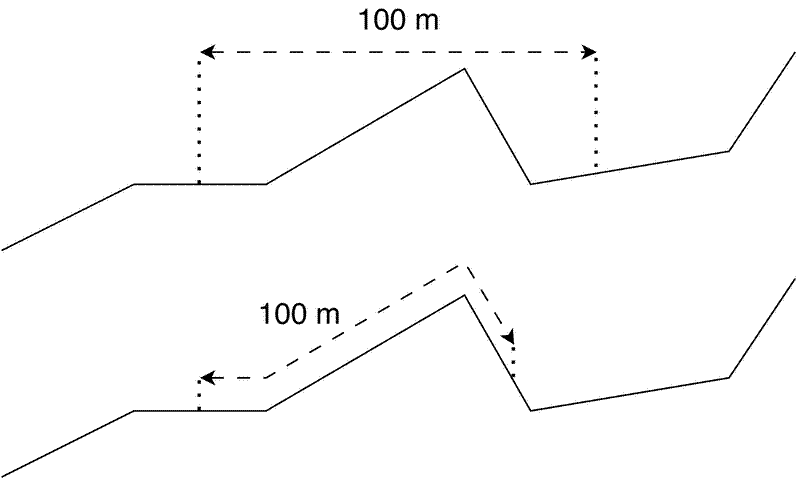
The area of plots should be measured relative to a planar projection. In other words, the distance between plot corners should be measured as a straight line as if looking down from above, not following the ground surface. While measuring plot area according to the ground surface is generally easier in the field, measuring relative to the ground surface will result in plots with a smaller planar area that may limit their use when matching with satellite data. Where dimensions of existing plots are measured relative to the ground surface, take extra care to precisely geo-reference the plot corners and all subplot corners.
Ideally orientate plots according to latitudinal north, not magnetic north. Again, this maximises potential overlap between the plot and whole pixels from satellite datasets.
Marking a plot
Setting up large plots can be time-consuming, but it is worth getting it right during plot establishment to save more work in the future. Here is a set of instructions on how to mark out a 50 m plot using tape measures:
- Start by identifying the centre location of the plot.
- Line 1: Using a compass, with adjustments for declination, walk from the centre point directly SW 35.35 m (sqrt(50^2 + 50^2) = 70.71 / 2 = 35.35). The SW corner is now fixed and ideally should not be moved.
- Line 2: Measure from the centre point NW 35.35 m.
- Line 3: Measure from the SW corner to the NW corner. This distance should be 50 m. If the distance is not 50 m, adjust the position of the NW corner so it is 50 m, ensuring that the length of the line from the centre to the NW corner remains 35.35 m.
- Line 4: Measure from the centre point NE 35.35 m.
- Line 5: Measure from the NW corner to the NE corner. Adjust the position of the NE corner accordingly.
- Line 6: Measure from the centre point SE 35.35 m.
- Line 7: Measure from the NE corner to the SE corner. Adjust the position of the SE corner accordingly.
- Line 8: Measure from the SE corner to the SW corner. This distance should be 50 m. If the distance is not 50 m, make minor adjustments to positions of the other corners.
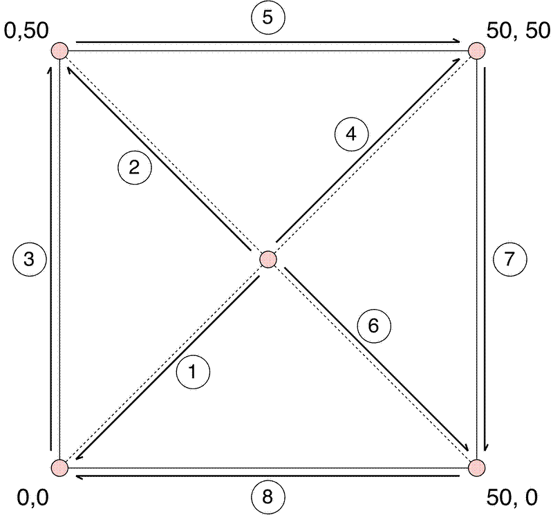
In dense forests where visibility is low you could instead sequentially mark out smaller quadrants of the plot using this method.
Add a robust and permanent marker at each plot corner. Concrete posts formed around reinforcing bar work well, buried so ~10 cm of the post is visible above the ground, with as much as possible below the ground. Bare re-inforcing bar also works, but can be harder to see and could be dangerous if somebody falls on it.
Where concrete and rebar are not allowed, for example where there is concern for the safety of animals which may fall onto the exposed rebar, consider using large metal plates which sit flush to the ground, with an anchor to stop them moving.
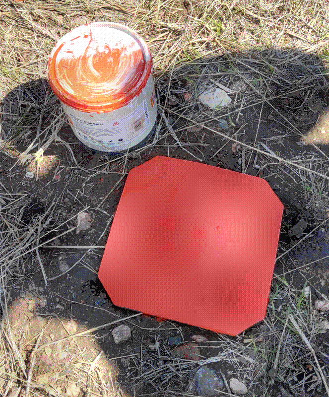
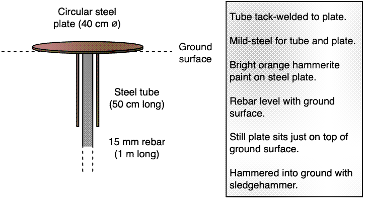
Consider spray painting plot markers in a conspicuous colour like fluorescent orange or green.
Add auxiliary markers at regular intervals around the perimeter of the plot, e.g. aligning with the corners of the subplots (see below). Make sure the perimeter markers look different to the corner markers so the location of the corner is not mistaken. Ideally also add auxiliary markers to the interior corners of the subplots. If possible make these different again from the perimeter auxiliary markers and the plot corners.
At some plots the risk of corner markers being removed by humans or animals means that an alternative approach is required. Metal posts or strong magnets can be buried completely and re-located using a metal detector. This is the most reliable method, provided the metal detector is of good quality and is being used by a trained operator. A differential Global Navigation Satellite System (GNSS) unit can be used to locate plot corners if multiple measurements are taken over the course of several days, removing any need for a permanent corner marker, but this limits future censuses to also using a differential GNSS unit. I do not recommend this approach. The position of plot corners can also be triangulated relative to known landmarks in the vicinity such as immovable rock outcrops or very large trees, but this strategy is risky if there is any chance that the landmarks will move, disappear, or their exact point location is ambiguous.
If using a handheld GNSS to record the locations of plot corners, collect waypoint-averaged corner locations over the course of several days or weeks, every time there is a visit to the plot, to account for systematic bias caused by satellite constellation. Even with a differential GNSS system, multiple measurements should be recorded over a long period of time. I recommend at least 15 measurements per corner. I recommend using the BIOMASS R package
which has the check_plot_coord() function, which can use multiple GNSS point estimates of each plot corner with information on the nominal plot dimensions to estimate the true location of plot corners.
Survey layout
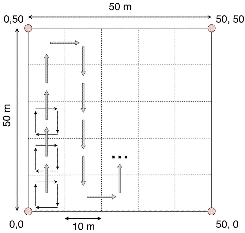
Divide the plot into a grid system. Commonly 20x20 m, sometimes 10x10 m if the vegetation is dense.
It is worth being meticulous in the layout of the subplot grid so that the corners of the subplots can be used as the origin points when mapping stems. Measuring a straight line over 10 m (maximum distance from an edge in a 20x20 m subplot) is much easier than measuring from the edge of the plot.
Ideally, record the GNSS location of all subplot corners in the same way as plot corners, with multiple measurements spread over several days or weeks. These subplot locations can also be used to refine the plot location.
Within each subplot, measure stems in a clock-wise fashion starting from the bottom left corner (normally SW) of the subplot.
Organise subplots in strips, moving up the first strip of subplots, then back down the next strip, and so on.
Stem mapping
Record the location of all measured stems within the plot.
Record the stem map coordinates of each plot corner and each subplot corner to allow the stem map to be orientated relative to the plot corners in global geographic space.
Measure stem location with a unit precision of 10 cm. Anything smaller than 10 cm is excessively laborious. Larger than 10 cm risks mixing up stems in the field during re-measurment based on the stem map.
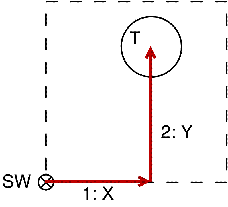
The location of each stem should be recorded relative to the SW corner of the subplot. Using tape measures, first measure along the X axis (West -> East), then measure up to the centre of the stem following the Y axis (South -> North).
If the tree is for example in top-right corner of the subplot, you could also measure relative to the top right corner (NE). To avoid having to calculate the real XY coordinate in the field by subtracting the measurement from the subplot dimensions, I instead record these measurements as negative values, which can then be corrected en masse in Excel after the fieldwork.
When to measure
In seasonally dry biomes, it may be easier to collect diameter measurements during the dry season when the ground layer is normally less thick, but this must be traded off against the ability to identify species if they are deciduous.
Research the site before planning a field campaign. Avoid periods of flooding, fire activity, etc.
Try to time tree inventory measurements to coincide with the collection of other datasets that might be used in comparison with the tree inventory data during analysis.
To reduce errors in diameter measurements caused by variations in stem water content, it is best to measure tropical forests toward the end of the wet season. Re-measurements of seasonal forests should be done at the same time of year as the previous censuses.
What to measure
Types of plant
This depends on the goals of the research, but I advocate for a maximalist approach which measures all arborescent perennial plants, hereafter referred to as trees. This broad definition includes what many think of as orthodox trees: dicot species which form a woody trunk by secondary growth. Additionally, the definition includes many other “tree-like” plants, included either because they produce woody tissue (e.g. Bamboo, lianas) or because they form a tree-like structure with an elongated stem supporting smaller branches and foliage (e.g. Banana plants). Below is a non-exhaustive list of arborescent plants which should be considered for measurement, despite either not being “tree-like” or woody-stemmed dicots:
- Palms (e.g. Cocos nucifera) – Arecaceae
- Tree-like members of Strelitziaceae (e.g. Ravenala madagascariensis)
- Bamboo (e.g. Phyllostachys spp., Dendrocalamus spp., Guadua spp.) – Poaceae
- Cycads (e.g. Cycas circinalis) – Cycadaceae, Zamiaceae
- Cacti (e.g. Pachycereus pringlei) – Cactaceae
- Banana plants (e.g. Musa acuminata) – Musaceae
- Papaya plants (e.g. Carica papaya) – Caricaceae
- Tree-ferns (e.g. Alsophila spp., Cyathea spp., Dicksonia spp.) - Cyatheales
- Lianas (e.g. Bauhinia guianensis, Saba comorensis)
Where species cannot be identified, note the growth-form of the individual if it is not an orthodox tree, e.g. one of the groups in the list above.
Minimum diameter threshold
The minimum diameter threshold defines the smallest stems that will be measured. The minimum diameter threshold should be the same for all plots in the site. Common minimum diameter thresholds are >= 5 cm and >= 10 cm. The minimum diameter threshold selected should ensure that at least 200 stems per hectare are measured. As mentioned above, if not enough stems are included within a 1 ha plot to make a representative estimate of AGBD, you may need to either increase the size of the plot, or decrease the minimum diameter threshold.
Edges
Stems should be measured if more than 50% of the base of the stem is inside the plot.
Where multi-stemmed trees straddle the edge of the plot, measure all stems on the tree, but note which stems are located outside the plot (i.e. more than 50% of the base of the stem is outside the plot).
Tagging
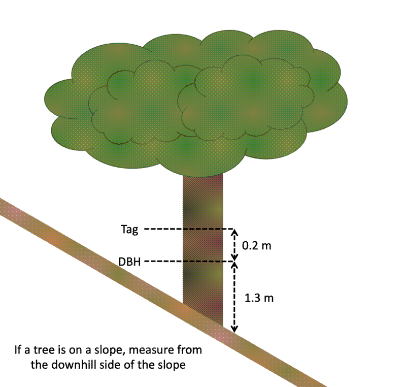
Nail tags into the stem 20 cm above the POM. Some other protocols recommend 30 cm. The important thing is that it’s consistent within the site, and not so close to the POM that it might cause damage to the stem where diameter is measured.
Hammer nails so that a few cm of nail is still visible, far enough that the nail penetrates the wood and is secure, but leaving as much space as possible for the tree to grow without “eating” the tag. Angle nails slightly downwards so the tag falls away from the tree. Otherwise, as the tree grows, the bark may “eat” the tag. I find that 60 mm steel nails (galvanised preferably to prevent rusting) hammered in 20-30 mm work well.
For stems < 5 cm diameter, use a loop of wire to attach the tag rather than a nail, as nails may damage the stem.
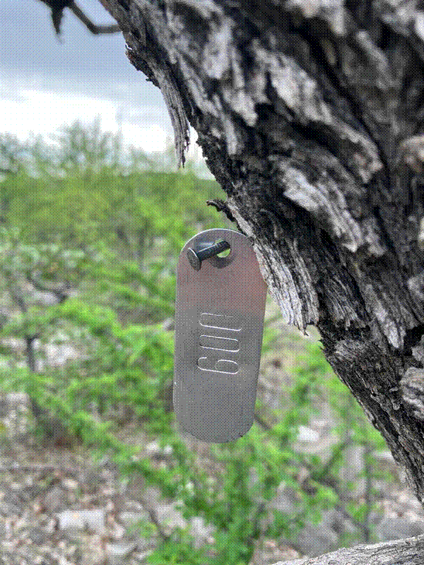
Have the diameter measurement person mark the POM with a chalk line, then the tagging person can measure the 20 cm distance above the POM to apply the tag. Some people also recommend painting the POM to aid re-measurement, but be careful that the paint does not cause damage to the stem. Some paints can cause lesions on certain trees, particularly those with thin bark.
Ideally, always place tags on one side of the stem. If a plot is near to a road, face all the tags away from the road. Having all the tags on one side of the tree makes it easy to know where to search for the tag during re-measurement.
Use a continuous number series of tags, do not use nested series’ with auxiliary numbers or letters for secondary stems. For new recruits found during re-measurement, use the next tag number in the series. Numbers and letters can easily be confused in the field, e.g. “6” and “b”, “8” and “B”. In subsequent censuses, choosing new letter and number combinations quickly becomes confusing, and increases the risk that a tag ID is accidentally duplicated.
If numbered tags can’t be bought, you can make them using thin zinc roof sheeting and a set of numbered punches. Cut the sheeting into tag sized pieces with tin snips. Poke a hole with a nail in the corner, then add the numbers using the punches.
On multi-stemmed trees, the tree ID of each stem should be recorded. This is normally the largest living stem on the tree, under the assumption that this stem is least likely to lose its tag and is most likely to survive until the next census.
If the goal is to quantify tree demographic rates and population dynamics, tags should be attached to every measured stem on multi-stemmed trees. In this case it is also useful to map each stem separately, to help identify stems in future censuses if the tags fall off, but this is not required. For estimates of plot-level AGBD change it is acceptable to tag only one stem on the tree, normally the largest living stem.
For multi-stemmed / resprouting trees, record the parent stem of each stem. E.g. if a stem emerges below the POM of a different stem, record the stem ID of that different stem. This may be different from the tree ID of the stem.
In dense stands I recommend visually marking stems once they have been measured in addition to the tag, for example with spray paint or flagging tape (make sure this is removed at the end of the census). This will make it easier for operators to check that all individuals within the plot were actually measured as expected.
Mortality
If stems are rooted in the ground they should be measured, even if they are dead.
If a stem is not rooted in the ground it can be classed as coarse woody debris and measured using a protocol designed for coarse woody debris (e.g. SEOSAW CWD protocol ).
These are the codes I recommend to indicate stem mortality status:
- “a” - alive, signs of life above the DBH measurement, e.g. the canopy of the stem is alive.
- “t” - topkilled, canopy of the stem is dead, but there are signs of life visible elsewhere on the stem.
- “d” - dead, no sign of life anywhere on the stem.
Stem condition and damage
These are the stem condition codes I use. These codes are meant to cover the majority of common stem conditions. The letters have been picked so that they are less likely to be confused when written hastily on paper. Most of these codes have been lifted from the SEOSAW manual, but there are some additions from RAINFOR, DryFlor and ForestGEO. I have also split up some of the codes in SEOSAW. E.g. “wounded or sick” was split into “wounded” and “sick”.
- “b” - broken (material above break is detached)
- “c” - has climbing or strangling plants in canopy
- “e” - buttressed
- “f” - fallen
- “g” - fluted
- “h” - hollow
- “j” - bark peeling or lost
- “k” - stem has bracket fungi
- “l” - leaning (>15deg)
- “m” - on a termite mound
- “n” - a new recruit
- “o” - stem is a resprout from an older stem. Where possible record the stem ID of this older stem.
- “p” - snapped (material above break is attached)
- “q” - the stem location is unknown and was not found (contrast with “v”)
- “r” - resprouting shoots are growing from the stem. Only if the shoots are smaller than the minimum diameter threshold, otherwise measure as a separate stem.
- “s” - standing
- “t” - stump (broken below POM)
- “u” - uprooted
- “v” - vanished (location of tree found but stem missing)
- “w” - stem is a liana
- “x” - rotten wood
- “y” - wounded
- “z” - sick (i.e. lost most leaves, discoloured foliage, drooping branches)
Similarly, here are the codes I use to refer to cause of damage. Obviously these reflect my experience working in fire-prone savannas with elephants.
- “a” - animals (not elephants, not insects)
- “e” - elephants
- “f” - fire
- “h” - humans (e.g. cut, ringbarked, broken or beehive)
- “k” - frost. This is difficult to ascertain.
- “l” - lightning
- “m” - termites
- “n” - neighbouring tree
- “o” - other (describe in damage_cause_notes)
- “q” - unknown. This should be used liberally. Only record damage cause if you are sure.
- “w” - wind
- “x” - climber weight
- “z” - climber competition
Diameter measurement
Diameter measurements on stems >= 5 cm diameter should be done using a diameter tape measure.
For stems < 5 cm diameter use vernier calipers, ideally with two perpendicular measurements. The buckle on diameter tapes means that the diameter of small stems is generally over-estimated.
Measure and tag all stems down to 1 cm below the minimum diameter threshold. E.g. if the minimum diameter threshold is 10 cm, measure all stems down to 9 cm diameter. These measurements can be filtered out later for analysis, and it ensures that small measurement errors do not lead to the false omission of individuals from the dataset.
Stem diameter should be measured at the default POM unless this does not provide a good representation of the diameter of the stem. Where the POM is moved ensure the height of the adjusted POM is recorded. Common reasons to move the POM include:
- Deformities - Stems that are deformed at the default POM, for example because of a wound, swelling, bark loss, cankers, cracks, burls, or a branch. Move the POM at least 10 cm below the base of the deformity.
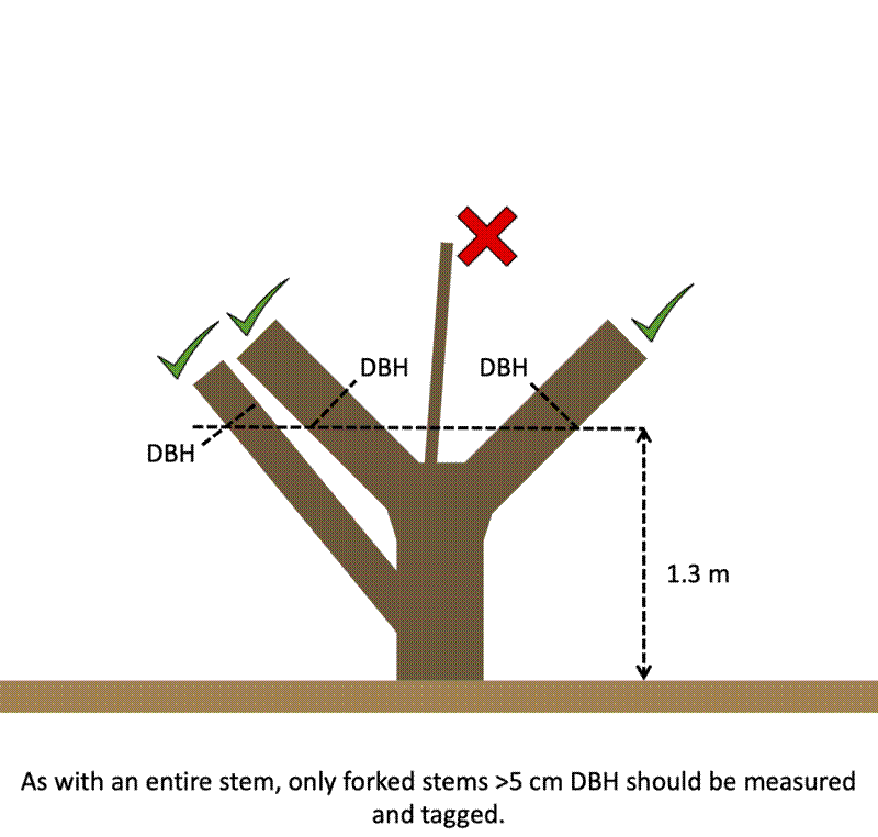
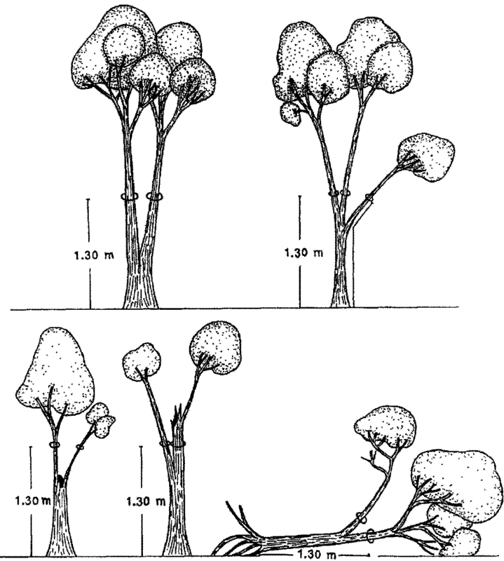
- Forked stems - Stems that fork into multiple stems at the default POM. Move the POM 30 cm below the bulge at the base of the fork.
- Buttresses and stilt roots - Move the POM 50 cm above the top of the buttress or the highest stilt root.
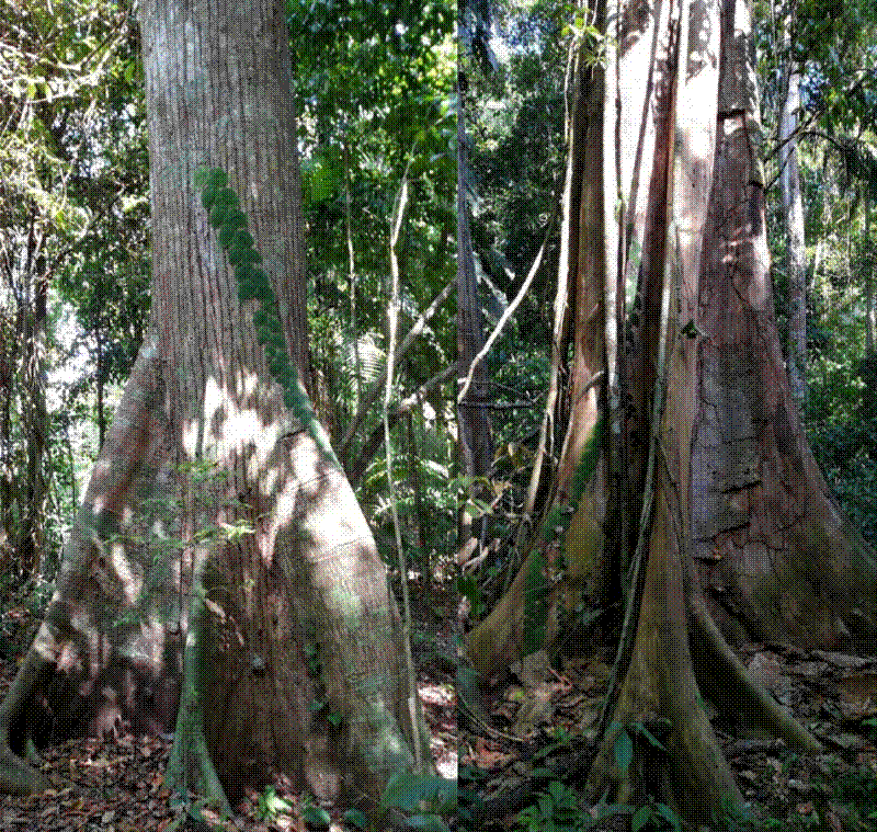
Where a stem is fluted along its length, measure using the default POM.
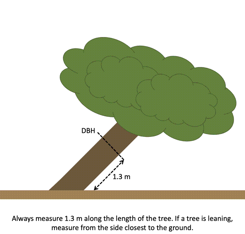
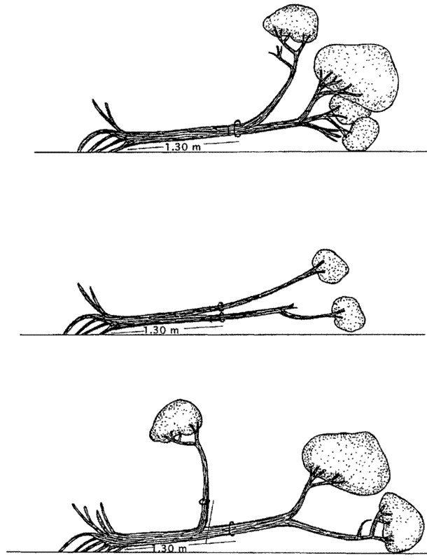
The POM should be measured along the length of the stem, not as the vertical height above the ground.
On leaning stems, the POM should be measured along the side of the stem closest to the ground.
On slopes, the POM should be measure on the downhill side of the slope.
Small climbers, epiphytes, roots, loose bark and debris should be lifted away from the POM before measuring the stem diameter. If the POM cannot be made clean, measure the stem diameter using calipers at two or more equally spaced points around the stem.
If a stem is broken and the break is on or below the POM, move the POM 2 cm below the base of the break. If the break is above the POM, measure the stem as normal. Record the location of the break as the height above the ground along the length of the stem.
On multi-stemmed trees, all stems reaching the minimum diameter threshold of the plot at the default POM should be measured.
Height measurement
If possible, measure the height of every stem in the plot.
Measure stem height up to the tallest living part of the stem.
I recommend using laser range finders for stems over three metres tall. For stems less than five metres tall, use a measuring stick.
On multi-stemmed trees, measure the height of individual stems, not of the tree as a whole.
Often it is not possible to measure every stem. In this case, aim to measure the heights of a stratified sample of stems.
Following Sullivan et al. (2018), I recommend sampling the largest stems of at least 50 trees per hectare. Measure the ten largest diameter trees in the plot, then measure a stratified random sample of 40 of the remaining trees across diameter size classes. Exclude trees which are leaning, rotten, broken, fallen, resprouted from an older base, or where significant parts of the canopy are dead. The stratified sample should be of sufficient size that the prediction interval from the model(s) is ≤ 1 m across the range of stem diameters. For this reason, measure stem height after all the diameter measurements have been completed.
For example, in R, with a dataframe (dat) of stems (stem_id) with diameter measurements (d), stem mortality status (status), stem modes (mode) and tree IDs (tree_id) within the plot:
n_per_dclass <- 8
n_dclass <- 5
n_largest <- 10
dat_fil <- dat %>%
  filter(
    !is.na(d),
    status == "a",
    !grepl(paste(c("b", "f", "l", "p", "t", "u", "o"), collapse = "|"), mode)) %>%
  group_by(tree_id) %>%
  slice_max(d, n = 1) %>%
  ungroup() %>%
  arrange(desc(d)) %>%
  {
    largest <- slice_head(., n = n_largest) %>%
      mutate(sample_group = "largest")

    remainder_strat <- slice_tail(., n = nrow(.) - n_largest) %>%
      mutate(d_class = ntile(d, n_dclass)) %>%
      group_by(d_class) %>%
      slice_sample(n = ceiling(n_per_dclass * n_dclass / n_dclass)) %>%
      ungroup() %>%
      mutate(sample_group = paste0("dclass_", d_class))

    bind_rows(largest, remainder_strat)
  } %>%
  dplyr::select(stem_id, sample_group)
Height measurements are generally very error-prone so regardless of the measurement apparatus used, take multiple height measurements. Exclude obvious outliers and keep taking measurements until you are confident in the average height estimate.
Species identification
Unless it is absolutely unambiguous across all plots within a site, I do not recommend using acronyms or shortened versions of species names on field data sheets. I have come across many instances where shortened species names can be confused with another species, leading to widespread errors in the dataset. For example, Pterocarpus angolensis and Pericopsis angolensis could both be shortened to PA, Pang, and so on. It is not enough to assign subtley different acronyms, e.g. “PTANG” for Pterocarpus angolensis and “PEANG” for Pericopsis angolensis, because somebody will inevitably confuse them in the field. Another example I’ve come across is ABPREC, which is meant to be Abrus precatorius, but was translated as Abarema precatorius, despite Abarema spp. not occurring at all within the site.
Ideally collect a herbarium voucher from every morpho-species found in the plots within a site. Note down which individual the specimen came from by the Tree ID.
Before fieldwork begins, ensure all relevant permits are secured (e.g. nationwide collection permit, protected area permit, genetic permit, export permit).
Record botanical sources used to assign taxonomic names, e.g. regional/national flora, trained botanist.
Use a well-trained botanist whenever possible, especially during the initial census. Ask the botanist to put together a field guide for the species present in the plot, especially groups of species that are difficult to differentiate.
Photographs of all characters useful for botanical identification should be taken, and all relevant characters and observations (e.g. presence and colour of exudate; colour of flowers; bark characteristics) should be included in collection labels. Voucher collections should be dried on the day of collection in an air drier.
Stopping work while herbarium specimens are collected slows everything down. You may want to save the botanical identification work until the diameter measurements have been completed. This will also give you a full picture of how many specimens need to be collected.
Quantifying error
Measurement errors occur throughout the data collection process:
- Diameter measurement
- Height measurement
- Stem mapping
- Taxonomy
- Stem mortality status
These repeat measurements should be conducted separately, after the main survey. It is recommended that the repeated measurements are conducted immediately after the main survey, and no more than six months after the main survey.
A quasi-random sample of stems can be generated by randomly selecting subplots. Measurements from the main survey should not be consulted when repeat measurements are taken. It is recommended that the same data collectors are used for the repeat measurements as for the main survey.
To minimise the influence of measurement errors on AGBD estimates, avoid using data from the first census where possible. Over subsequent censuses it is common that many errors are fixed and the dataset becomes more refined.
Re-measurement
Re-measuring plots is normally done on a 3-5 year time-scale. Long enough that stem diameter growth is larger than the error on diameter measurements.
Conduct the second census (i.e. first re-census) sooner than normal. During the second census many issues in species identity, stem mapping, and diameter measurement can be caught and retro-actively corrected. If the census interval is too long, trees will start to die and so cannot be checked in the second census.
Between censuses it might still be worth doing maintenance on the plot, particularly replacing plot corners if they become obstructed or go missing.
Tagging new recruits with the next number in the sequence of tags means that over the course of a few censuses, the tag order quickly becomes complicated. Create a “measurement order” column for your data to specify the order in which stems should be measured within the plot. Record the position of new recruits in this stem order sequence so that when new datasheets are created the order of stems on the datasheet will resemble the real-world order of stems in the field.
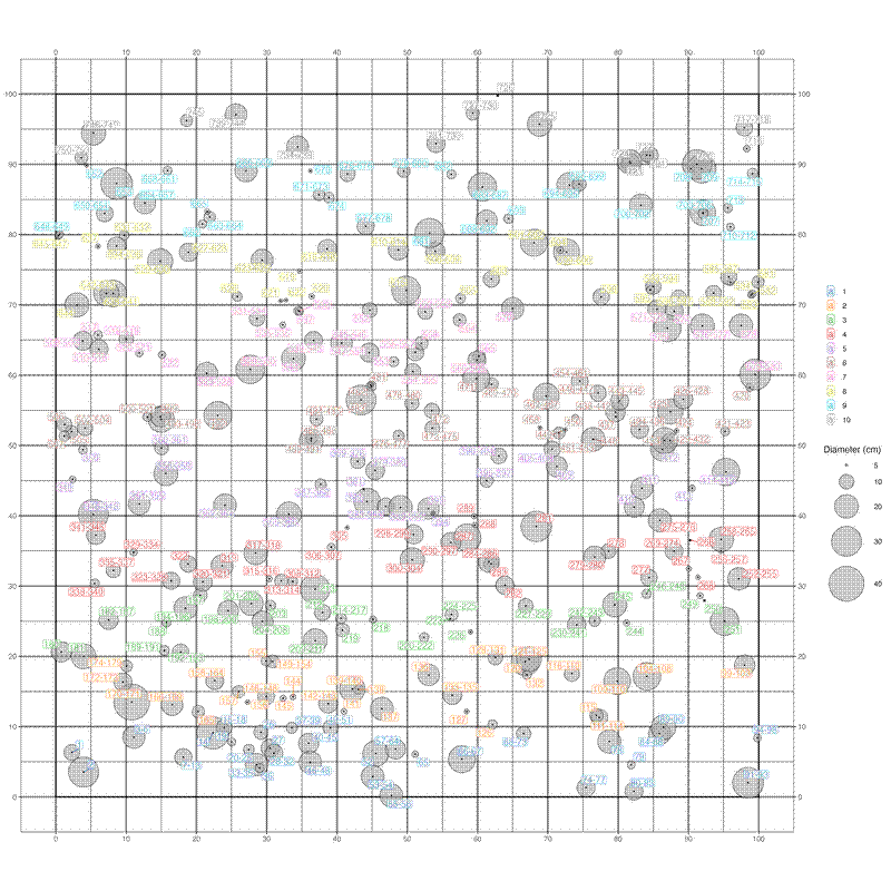
Generating a stem map and printing on a large sheet of A3 paper, or keeping a copy on a tablet computer can be very helpful for re-measurement, especially when re-locating subplot edges. Here is some code I use to generate pretty stem maps in 100x100 m plots:
# Packages
library(dplyr)
library(ggplot2)
library(ggrepel)

# Import data
s <- read.csv("./stems.csv")

# Clean data
s_clean <- s %>%
  filter(
    plot_id == "NOC_7",
    !is.na(subplot_id),
    !is.na(x_grid),
    !is.na(y_grid)) %>%
  group_by(subplot_id, tree_id) %>%
  summarise(
    species = first(species_name_clean),
    tag_id = paste0(unique(tag_id), collapse = ","),
    x_grid = mean(x_grid, na.rm = TRUE),
    y_grid = mean(y_grid, na.rm = TRUE),
    diam = max(diam, na.rm = TRUE)) %>%
  ungroup() %>%
  mutate(
    diam = ifelse(!is.finite(diam) | is.na(diam), 5, diam),
    subplot_id = factor(subplot_id, levels = sort(unique(subplot_id))),
    tree_tags = case_when(
      grepl(",", tag_id) ~ paste0(sub(",.*", "", tag_id), "-", sub('.*,', '', tag_id)),
      TRUE ~ tag_id))

species_top10 <- sort(table(s_clean$species), decreasing = TRUE)[1:10]

s_clean_labs <- s_clean %>%
  mutate(species_top10 = ifelse(species %in% names(species_top10), species, "Other"))

# Create polygons for plot outlines
po <- data.frame(area = 1.0, x = c(0,0,100,100), y = c(0,100,100,0))

# Define colour scheme for subplots
pal <- c("#1F77B4", "#FF7F0E", "#2CA02C", "#D62728", "#9467BD",
         "#8C564B", "#E377C2", "#BCBD22", "#17BECF", "#7F7F7F")

# If necessary, replicate colour palette to number of subplots
pal_rep <- rep(pal, length.out = length(unique(s_clean_labs$subplot_id)))

# Create plots
out <- ggplot(s_clean_labs, aes(x = x_grid, y = y_grid)) +
    geom_polygon(data = po, aes(x = x, y = y),
      colour = "black", fill = NA) +
    geom_point(aes(size = diam), shape = 21, fill = "darkgrey", alpha = 0.6) +
    scale_size(name = "Diameter (cm)",
      range = c(1, 20),
      breaks = c(5, 10, 20, 30, 40, 60, 80, 100)) +
    geom_point(colour = "black", size = 0.25) +
    geom_label_repel(aes(label = tree_tags, colour = subplot_id),
      label.padding = unit(0.08, "lines"),
      alpha = 0.7,
      max.overlaps = Inf) +
    coord_fixed() +
    scale_x_continuous(
      name = NULL, breaks = seq(0,100,10),
      sec.axis = dup_axis(name = NULL, breaks = seq(0,100,10))) +
    scale_y_continuous(
      name = NULL, breaks = seq(0,100,10),
      sec.axis = dup_axis(name = NULL, breaks = seq(0,100,10))) +
    scale_colour_manual(name = NULL, values = pal_rep) +
    theme_bw() +
    theme(legend.position = "right") +
    ggtitle(unique(s_clean_labs$plot_id)) +
    theme(
      plot.title = element_text(
        hjust = 0.5, vjust = -0.5, face = "bold", size = 20),
      panel.grid = element_line(
        linewidth = 1,
        colour = alpha("black", 0.5)))

# Save plots to file
ggsave(out, width = 15, height = 15, file = "stem_map.png")
