Mapping GPX tracks from AAT for Android, in R

I stopped using Strava to track my cycle rides, because I didn’t feel comfortable giving away all that GPS data to a third party. I know lots of other things I do give away my location, but this is a small step in the right direction. It also prompted me to play with new GPS tracking apps.

The one I have settled on is called AAT , which is a lovely brutalist piece of open source software that is designed around tracking cycling.

It stores tracks as GPX files, which can then be manipulated and plotted in other softwares. In this case, I wanted to use R. The script is below and here and an example GPX file from AAT can be found here .

Note that you may have to install ggmap from the github repository like this: devtools::install_github("dkahle/ggmap"), as the CRAN mirror is often way behind.

# Packages ----
library(rgdal)  # readOGR(), ogrListLayers()
library(ggplot2)  # ggplot()
library(ggmap)  # get_map(), ggmap()

# setwd ----
setwd("~/tracks")

# Import file ----
# Find out what layers are in the file
(layers <- ogrListLayers("2018_04_19_0.gpx"))

# Import the points layer, which contains elevation data
track_points <- readOGR("2018_04_19_0.gpx", layer = layers[5])
# Import the tracks layer as a spatiallinesdataframe

# Test plot
plot(track_points)

# Transform data to data frame for plotting ----
# Create data frame from spatial object
track_df <- data.frame(track_points@coords, 
	track_points$ele, 
	track_points$time,
	track_points$track_seg_point_id)

# Rename columns
names(track_df) <- c("lon", "lat", "elev", "time", "seg_id")

# Convert time to posixCT
track_df$time_posix <- track_df$time %>%
	as.POSIXct(., format = "%Y/%m/%d %H:%M:%S ")

# Create plots ----
# Create elevation plot
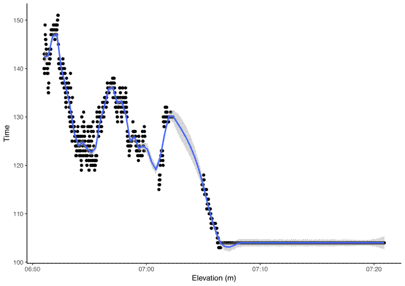
(elev_plot <- ggplot(track_df, aes(x = time_posix, y = elev)) + 
	geom_point() + 
	geom_smooth(method = "loess", span = 0.1) + 
	scale_x_datetime() + 
	theme_classic() + 
	xlab("Elevation (m)") + 
	ylab("Time"))

# Plot map using ggmap
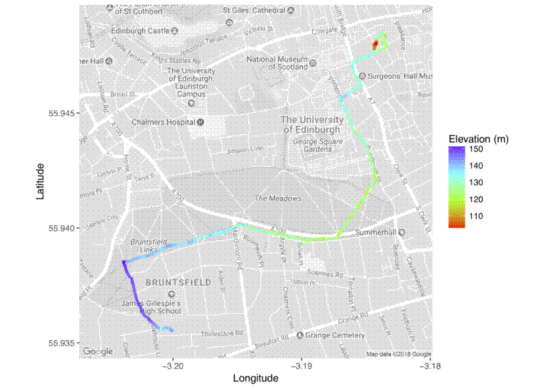
goog_map <- get_map(location = track_points@bbox, 
	zoom = 15, 
	maptype = "roadmap", color = "bw")

(route_map <- ggmap(goog_map) + 
	geom_path(data = track_df,
	aes(colour = elev), size = 1.5) + 
	scale_color_gradientn(colours = rainbow(4)) +
	guides(colour = guide_colourbar(title="Elevation (m)")) + 
	xlab("Longitude") + 
	ylab("Latitude"))

The script outputs an elevation plot and a map which shows the track, coloured by elevation.