Most tree inventory plots have a minimum stem diameter threshold. Tree stems with a diameter lower than this threshold are not measured, because they are often too numerous to measure, and they contribute comparatively little to the total woody biomass of the plot.
Different sites have different minimum stem diameter thresholds, though 5, 10 and 20 cm are common. If we are going to compare woody biomass stocks across sites, how do we account for this difference in methodology, which could otherwise lead to lower estimates of the biomass stock where the minimum stem diameter threshold is higher?
One option would be to do nested sub-sampling, where smaller stems are measured within a small portion of the total plot area. Then you multiply up the biomass of small stems within the smaller subplots to the area of the whole plot. This method assumes that the spatial distribution of small stem biomass is consistent across the plot. Many plots don’t do this nested sub-sampling, but I believe it is the best way to deal with this problem.
Another option is to predict the abundance of stems in smaller size classes within the plot by extrapolating the stem size distribution. Stem size distributions in undisturbed forests often follow something close to a Weibull distribution .
Fitting a basic Weibull distribution to the data is not appropriate, because we know that it’s truncated at the minimum stem diameter threshold. I wrote some functions in R that fit a truncated Weibull distribution, then predict the abundance of stems in smaller size classes from this fitted distribution:
First create some fake data with a known Weibull distribution, for testing:
# Create fake data with known Weibull distribution
D <- rweibull(100000, shape = 1.2, scale = 50)

# Truncate to lower bound
Dt <- D[D > lower_bound]
Then define basic distribution functions for a truncated Weibull distribution, using the truncdist package:
# Define distribution functions for truncated Weibull
dtweibull <- function(x, shape, scale, lower, upper) {
  truncdist::dtrunc(x, "weibull",
    a = lower, b = upper,
    shape = shape, scale = scale)
}

ptweibull <- function(q, shape, scale, lower, upper) {
  truncdist::ptrunc(q, "weibull",
    a = lower, b = upper,
    shape = shape, scale = scale)
}

# Define function to fit Weibull distribution to data
tweibull_fit <- function(x, shape, scale, lower, upper) {
  fitdistrplus::fitdist(x, "tweibull",
    start = list(
      shape = shape,
      scale = scale),
    fix.arg = list(
      lower = lower,
      upper = upper))
}
And finally a function to fit the model and use it to predict stem size abundance in lower size classes:
# Define function to predict distribution outside truncation
tweibull_pred_fun <- function(x, lower = Inf, upper = Inf, bins) {
  # Rescale data by mean
  scale_val <- mean(x)
  x_scale <- x / scale_val
  bins_scale <- bins / scale_val
  lower_scale <- lower / scale_val
  upper_scale <- upper / scale_val

  # Estimate starting parameters of Weibull distribution
  fit_est <- unname(MASS::fitdistr(x_scale, "weibull")$estimate)

  # Fit truncated Weibull, using full Weibull parameters as starting
  fit_trunc <- tweibull_fit(x_scale, fit_est[1], fit_est[2],
    lower_scale, upper_scale)

  # Extract parameters from truncated Weibull fit
  var_arg <- as.list(fit_trunc$estimate)
  fix_arg <- as.list(fit_trunc$fix.arg)

  # Get cumulative probabilities at bin edges
  probs <- pweibull(bins_scale, var_arg$shape, var_arg$scale)

  # Calculate bin probabilities (differences between successive CDF values)
  bin_probs <- diff(probs)

  # Get total probability within non-truncated region
  probs_trunc <- sum(
    bin_probs[bins_scale >= lower_scale & bins_scale < upper_scale],
    na.rm = TRUE)

  # Multiply up
  bin_probs_mult <- (1 / probs_trunc) * bin_probs

  # Multiply bin probabilities by total number of values
  abundance_bins <- length(x) * bin_probs_mult

  # Construct dataframe
  out <- data.frame(
    bin = bins[-length(bins)],
    abund = abundance_bins)

  return(out)
}
Then run the function on the testing data:
fit_trunc_df <- tweibull_pred_fun(
  x = Dt,
  lower = lower_bound,
  upper = upper_bound,
  bins = seq(0, max(Dt), 5))
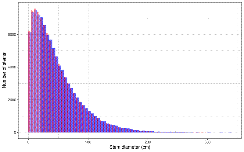
And compare the predicted data to the original data. Blue is the original non-truncated data, with the truncated training data in dark blue. Red is the estimated distribution from the truncated data:
# Create test plot
ggplot() +
  geom_histogram(aes(x = D), fill = "blue", binwidth = 5, alpha = 0.4, boundary = 0) +
  geom_col(data = fit_trunc_df, aes(x = bin, y = abund),
    fill = "red", width = 2, alpha = 0.5, just = 0) +
  theme_bw() +
  labs(
    x = "Stem diameter (cm)",
    y = "Number of stems")
